Measuring 3pt Shooting Ability With a Multilevel Model

Over the past couple of months I took an awesome class on categorical data analysis. Although it may not sound like it, this sort of data analysis has a lot of application to basketball, as it covers analyzing and building models for things like odds of events, probabilities of success, etc.

Although we didn’t cover it in class, the final chapter in our book by Alan Agresti covered multilevel models (otherwise known as mixed or random effects models). This finally allowed me to start to piece together the large treatment on this topic by Andrew Gelman and Jennifer Hill in their book on regression and multilevel models.

(Hopefully these references provide some reading for those interested in the details of these models.)

An example by Agresti on free throw shooting inspired me to see how we might apply a basic multilevel model to other NBA statistics. I chose 3pt shooting.

The Purpose of a Multilevel Model

The best way for me to explain the purpose of a multilevel model (with respect to sports, at least) is to liken it to a model-based regression to the mean.

By grouping similar players together, we take advantage of what we know about the average player from this group of players with the actual data we collect for each individual player. Like regression to the mean, this allows us to make sense of small samples and intelligently pool the group and individual-specific data together.

Since it’s model based, one advantage of this type of analysis over regression to the mean is that we can more easily quantify effects of the game, like home court advantage, that we might otherwise have a hard time quantifying.

There are more complex multilevel structures that I hope to understand in the future that will hopefully allow for controlling for other aspects of the game. Although not considered here, we might want to control for quality of opponents when rating individual player ability. This is simply one of many things we might want to control for that a more complex model structure may provide over the model presented here.

The Data Used for This Model

The models presented below were fit to a data set containing all 3pt shots attempted from a reasonable distance during the 02-03 through 08-09 seasons. This data set is grouped by the following categories:

• Season
• Player Position: from 1 through 5 to denote PG, SG, SF, PF, and C
• Player Name
• Player Age: as of June 1st prior to the start of the upcoming season
• Home vs Away
• Corner 3pt shots vs Other 3pt shots: a corner 3pt shot is defined to take place within 10ft of the baseline

Here is a sample from the data set that shows Kobe Bryant’s 3pt shots from the 08-09 season:

Season,Position,Name,Age,Game Location,Shot Location,Makes,Misses
2008,2,Kobe Bryant,30,A,corner3,7,7
2008,2,Kobe Bryant,30,A,other3,74,135
2008,2,Kobe Bryant,30,H,corner3,6,14
2008,2,Kobe Bryant,30,H,other3,59,99

Each player’s position is held constant for each season and taken to be the position listed from the most recent season. The position data comes from doug’s stats and the date of birth data comes from database basketball and NBA.com.

The Basic Model Structure

This model considers 3pt shots that are grouped by player. A separate model was fit for each position. The purpose of this model is to estimate each player’s ability while controlling for things like home court advantage, corner 3pt shots vs other 3pt shots, and age effects.

The models below were fit with R using glmer() from the lme4 package.

The Model Fits

PG: logit^-1( -1.40 + 0.02(home) + 0.11(corner3) + 0.053580(age) – 0.000911(age²) )

SG: logit^-1( -0.60 + 0.03(home) + 0.11(corner3) )

SF: logit^-1( -0.64 + 0.04(home) + 0.12(corner3) )

PF: logit^-1( -3.12 + 0.03(home) + 0.10(corner3) + 0.170527(age) – 0.002965(age²) )

The fit for centers does not appear to be that useful. Most centers don’t take that many 3pt shots. It might be better to group centers of interest with power forwards, but for now we’ll ignore these players (sorry Mehmet and Sheed).

All of the coefficients for the fits listed above are significant at the 0.10 level, except for the coefficient for home in the PF fit. It’s about what we would expect it to be at 0.03, so it seems reasonable to leave it in the model.

Interpreting These Fits

First I want to note that failure to converge warnings were encountered when including the age effects in the SG and SF fits, which is the primary reason why we are not controlling for those variables for shooting guards and small forwards. I’ve been unable to resolve this issue, so for now we will assume these players do not have an age effect for their 3pt shots.

That said, here is how we might interpret the effects in these fits:

• Home Court Advantage: We estimate the odds of making a 3pt shot at home are 2% higher than the odds of making a 3pt shot on the road for point guards, controlling for player ability, corner 3pt shots vs other 3pt shots, and age. We estimate this effect to be 3%, 4%, and 3% for shooting guards, small forwards, and power forwards, respectively. From a practical standpoint, we find no evidence that any one position has a higher home court advantage over any other position.
• Corner 3pt Shots: We estimate the odds of making a 3pt shot from the corner are 11.6% higher than the odds of making all other 3pt shots for point guards, controlling for player ability, home court advantage, and age. We estimate this effect to be 11.6%, 12.8%, and 10.5% for shooting guards, small forwards, and power forwards, respectively. Like home court advantage, there is no evidence that any one position has a higher corner3 effect than any other position.
• Aging Curve: We estimate that the peak age for 3pt shooting ability for point guards and power forwards is when these players are 29 years of age.
• Home 3pt FG%: We estimate that the average 29 year old’s non-corner 3pt FG% at home is 35.6% for point guards, 36.1% for shooting guards, 35.4% for small forwards, and 34.6% for power forwards.

The Player Effects

Of ultimate interest here is the player effects that quantify the player ability. Before diving into the numbers, I think it’s worth noting what exactly player ability means in the context of this model. Because we only control for home court advantage, corner 3pt shots vs other 3pt shots, and age, the player ability component is essentially a combination of true player talent, coaching, teammates, opponents, and other things like actual shot selection. A player that suddenly takes nothing but wide open 3pt shots is likely to overperform what we might predict from this model, or underpform if they were able to take the opposite action and only attempt heavily contested 3pt shots. This shot distribution is surely to be affected by coaching, teammates, and opponents.

With that in mind, the following spreadsheet lists 95% confidence intervals for the 3pt shooting ability of each player at home, 29 years of age, and where the uncertainty comes only from the error in the measured ability of each player. The uncertainty associated with the mean intercept, home court advantage, corner3, and age effects are not taken into account.

Spreadsheet: Multilevel Model: Estimated 3pt Ability

Aging Curve Examples

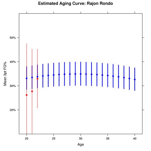
Rajon Rondo has been in the news a lot lately, so I figure he is as good a player as any to take part in showing the estimated aging effect for point guards.

In the graph below the blue represents the predicted mean 3pt FG% for Rajon Rondo weighted based on his actual shot distribution from all seasons in this data set. The red represents the actual estimated mean 3pt FG% for Rajon from those seasons, also weighted based on his actual shot distribution from all seasons in this data set. The dots represent the median, while the lines illustrate the 95% confidence interval for this mean 3pt FG%.

The uncertainty shown is only for the uncertainty in the actual measured player effect. The uncertainty on the age coefficients gives us fairly wide intervals to work with, so this uncertainty has been removed for clarity in the graph. This highlights the lack of precision for the estimated aging curve, even though the coefficients are statistically significant.

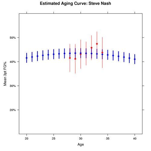
For a comparison, here is Steve Nash’s estimated aging curve:

There are two things to take away from this comparison. First, we have more data on Steve Nash, so the uncertainty around his ability is smaller than the uncertainty around Rondo’s ability. This is shown by the smaller bars in Nash’s graph.

Second, the aging effect for point guards is estimated to be fairly small. By that I mean the curve is not very steep, so although the curvature exists, we estimate it to be a fairly flat curve.

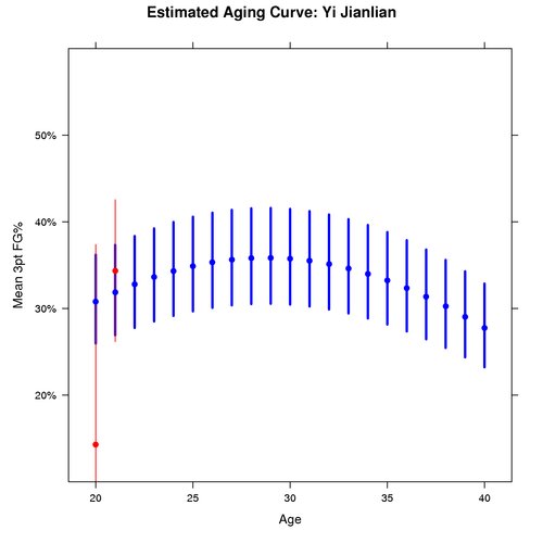
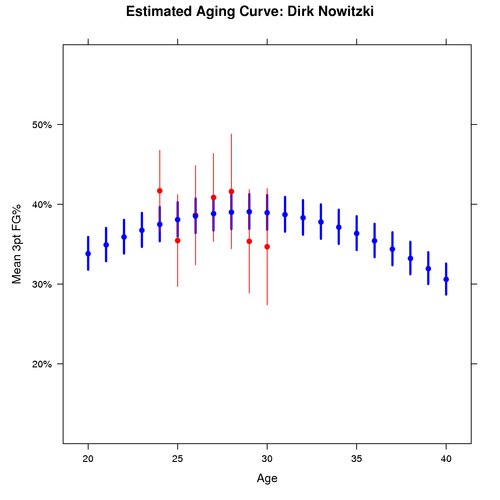
Point guards, however, are not the only position we estimated aging effects for. Here are similar graphs comparing a young power forward to a veteran power forward:

Like Rondo, there is more uncertainty around Jianlian’s ability than Nowitzki’s. Another comparison to the point guards comes in the shape of the curve. As the graphs show, the estimated curve for power forwards is steeper than the estimated curve for point guards.

Recreate These Results

To recreate these results with the R and data files listed below, you will need to install the arm package and its associated dependencies. One easy way to do this should be to run the following command from your R console:

install.packages(“arm”, dependencies=TRUE)

Once you have these packages, you’ll need to download these files:

• multi_3pt.R: By default, this R script simply fits the models above. You can then use summary(fits[[i]]) to see the results, where i = 1, 2, 3, or 4. Edit the code where you see the first if (0) statement to create the graphs above. Edit the code where you see the second if (0) statement to create the CSV file used to generate the spreadsheet above.
• raw_3pt.csv: This CSV data file contains the data as defined in the data section at the beginning of this post.

Summary

This is my first attempt at using a multilevel model with NBA, so there is certainly a mistake or two lying around somewhere. 🙂

I used the simplest structure possible for this model, so my hope is that future research in this area will allow for different groupings. One such grouping would ideally be at the team (or coach?) level.